The Fehlberg Method - Example

Problem A1 from W.H. Enright & J.D. Pryce (Two Fortran Packages For Assessing Initial Value Methods, ACM Trans. On Mathematical Software, Vol. 13, No. 1, 1987, pp 1-27) was solved using the RK-Fehlberg method. The ODE’s for the IVP are:

 


                                                                                                                                         
 with initial values of 1 for all y’s. A constant step size of 1E-2 was used. The results are plotted below.

 



 

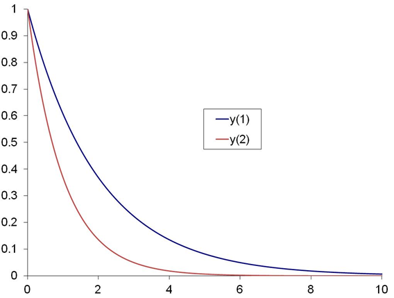
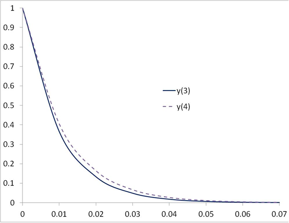
 The vastly different exponent factors of y3 and y4 (i.e., -100 and -90) compared to those of y1 and y2 (-0.5 and -1.0) result in quicker decay in the solutions for y3 and y4. For clarity, the results above are shown in two different plots with different scales for the abscissa.

The higher the exponent factor of an ODE, the smaller the step-size has to be to converge to a solution.