The Lotka-Volterra Predator-Prey Problem

Relationships between predators and prey are modeled using the Lotka-Volterra (LV) ODEs. The generalized form of the LV equations is:





Y1 represents the number of prey, and y2 the number of predators. Using the initial values and constants from Atkinson et al (Numerical Solution of ODEs), the Runge Kutta Merson method was used to solve the equations.

The Variable step Method of Fehlberg

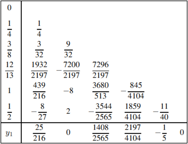
In order to incorporate a variable step algorithm for the Fehlberg’s method, an equation for error estimation has to be included. The Butcher tableau (ref: Hairer, Nørsett & Wanner, Solving ODEs, Vol. 1, Non-stiff problems) with the ycap coefficients are:

 

The generalized RK method can then be used with the Kaps-Rentrop algorithm for adaptive step size to solve ODEs.                                                                                                                       

The Brusselator Problem

The Brusselator is a class of ODE’s that describe the autocatalytic reaction. The ODE’s that define the Brusselator as presented in Hairer et al (Numerical Solution of ODEs, Vol 1, Non Stiff Equations) are:

    

 

with initial values y1(0)=1.5 and y2(0)=3. The RK-Merson method with the Kaps & Rentrop variable step size algorithm was used to solve the Brusselator problem. An initial step size of 0.001 with a TOL of 0.001 was used.

 The results are shown below. The first figure shows the solutions of y1 and y2 as a function of x. The power of the variable step size is evident from the “dots” in the figure. Extremely small steps are required to initiate the numerical process close to start (at t=0), while fairly generous step sizes can be used as the integration progresses along. Had a fixed step size algorithm been used for the Brusselator, the step size would have to be small all along to avoid numerical instabilities, and thus increases the computation cost significantly.

 

 

Kaps-Rentrop’s Variable Step Size Procedure

The need for a variable stepsize control becomes evident when solving a series of ODE’s that have varying settling times for the solution. The requirement for stepsize is limited by the variable that has the shortest settling time, while the small step may be an over kill for the variables with slower settling times. Press et al (Numerical Recipes, The Art of Scientific Computing) very beautifully state that “many small steps should tiptoe through treacherous terrain, while a few great strides should speed through smooth uninteresting countryside”.

P. Kaps & P. Rentrop (Generalized Runge Kutta Methods of Order Four With Stepsize Control for Stiff ODE’s, Numerical Mathematics, vol. 33, 1979, pp. 55-68) have suggested the following stepsize control for adaptive steps in the integration of ODE’s.

Error estimation (and control) is performed by using two separate calculations with coefficients from the Butcher table as described in the Merson’s method. Having calculated y(n+1) and ycap(n+1),

1-      Define a suitable scaling factor

2-      Calculate the local Error estimate, EST 

 

 3-      Given a user supplied tolerance TOL, the new step size can be calculated as

 

 4-      The following algorithm can then be used for stepsize control:

 Do Until EST <= TOL

-       Calculate hnew
-       Recalculate y(n+1) and ycap(n+1) with hnew

At each stage of the iterative process, hnew is not accepted until EST<=TOL. hnew is progressively reduced in size until EST<=TOL. Once this condition is met, the same formulation for hnew is used one more time to advance to the next step.

Kaps & Rentrop suggest C=1 for the scaling vector, and a safety factor SF = 0.9 to conservatively guess on the new step. They also suggest bounding the stepsize with a min and max delimiter, as outlined in the Euler’s variable step algorithm.

The RK-Merson Method

R.H. Merson (An operational method for the study of integration processes, Proc.
Symp. Data Processing, Weapons Research Establishment, Salisbury, Australia, 1957, pp 110-125) came up with an RK formulation of order 4. The Butcher tableau for the Merson’s method (ref: Hairer, Nørsett, Wanner, Solving ordinary differential equations, vol.1. Nonstiff problems, 2nd ed) is shown below:



Notice a second row (ycap1) at the end in the tableau. By using a 4th order formulation, followed by a 5th order estimate for the new coefficients in the last row, an error estimate can be calculated.

The generalized Butcher tableau for with error estimation then becomes



The calculations for ki’s and y(n+1) remain the same from the Generalized RK procedure. The error estimation equation is defined by

 

The difference between the two values of y then serves as an estimate of the error. A variable step algorithm can then be developed based on the error estimate, similar to the one presented for the Euler’s method.

The Nystrøm’s Method – An Example

Problem C1 (Class C: Non-linear coupling) from W.H. Enright & J.D. Pryce (Two Fortran Packages For Assessing Initial Value Methods, ACM Trans. On Mathematical Software, Vol. 13, No. 1, 1987, pp 1-27) was solved using the RK-Nystrøm’s method. The ODE’s for the IVP are:






with initial values of 1 for all y’s. A constant step size of 1E-2 was used. The results are plotted below.

The RK-Nystrøm Method

In “A History Of Runge Kutta Methods” (Applied Numerical Mathematics, 20, 1996, pp 247-260), J.C. Butcher presents a set of coefficients for a 5^th order RK method as derived by Kutta. The tableau is shown below:

  

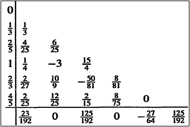
However, Butcher indicates that Kutta’s 5^th order coefficients had slight errors, which were subsequently corrected by Nystrøm in 1925. The method with these coefficients are more commonly known as the RungeKutta – Nystrøm method. The tableau for the Nystrom coefficients are :

 

 The Generalized RK formulation can then be used to solve a set of ODE's.

The Fehlberg Method - Example

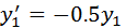
Problem A1 from W.H. Enright & J.D. Pryce (Two Fortran Packages For Assessing Initial Value Methods, ACM Trans. On Mathematical Software, Vol. 13, No. 1, 1987, pp 1-27) was solved using the RK-Fehlberg method. The ODE’s for the IVP are:

 


                                                                                                                                         
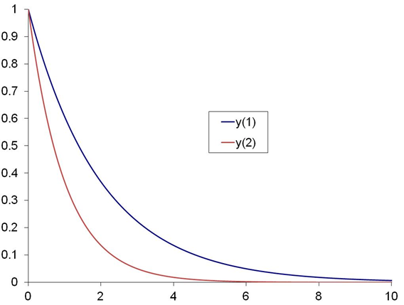
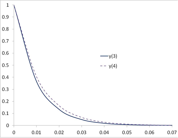
 with initial values of 1 for all y’s. A constant step size of 1E-2 was used. The results are plotted below.

 



 

 The vastly different exponent factors of y3 and y4 (i.e., -100 and -90) compared to those of y1 and y2 (-0.5 and -1.0) result in quicker decay in the solutions for y3 and y4. For clarity, the results above are shown in two different plots with different scales for the abscissa.

The higher the exponent factor of an ODE, the smaller the step-size has to be to converge to a solution.

The Fehlberg Method

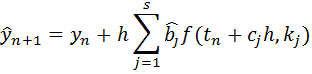
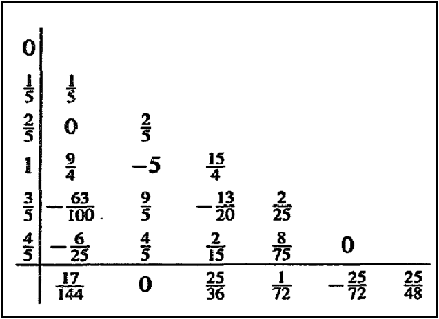
Several authors have researched on determining various sets of coefficients for higher order RK methods. Erwin Fehlberg’s NASA publications from the 1960’s (Classical Fifth, Sixth, Seventh and Eighth Order Runge Kutta Formulas With Step Size Control, NASA TR-R 287, 1968, and Low Order Runge Kutta Formulas With Step Size Control And Their Application to Heat Transfer Problems, NASA TR-R 315, 1969) present one such set of coefficients for RK methods of orders 4 and higher. The Fehlberg coefficients for RK4 are presented in the table below (ref: Hairer, Nørsett & Wanner, Solving ODEs, Vol. 1, Non-stiff problems). The generalized formulation can once again be used to solve the initial value problem.

                                                                                                                                       

Generalized Runge Kutta Formulation

For RK methods of order 4 and higher, the inter-stage vectors (k’s) can be represented using the following formulation (Atkinson et al, Numerical Solution of ODE’s):

    

The solution at t(n+1) is given by

 

J.C. Butcher (Numerical Methods for ODE’s, 2^nd Edition) invented the “Butcher tableau” methodology of representing the coefficients a(i,j), b(j) and c(j) for the Runge Kutta methods. The general format of such a tableau is

 

 The Butcher tableau for the most popular RK4 method thus becomes:

                                                                                                           

The use of the Butcher tableau, along with the generalized formulation from Atkinson, provides an easy methodology for numerical integration of ODEs.

Runge Kutta 4 - A Numerical Example

Oscillations and vibrations of structural elements are commonly represented as a 2^nd order ODE (derived from Newton’s law). In his paper, Piche (An L-stable Rosenbrock Algorithm for Step-By-Step Time Integration in Structural Mechanics, Computational Methods in Applied Engrg., Vol 126, 1995, pp 343-354) presents one such example of a two-degree of freedom mass-spring-damper system with the following ODEs:

 
with the initial values and constants defined as:

 

Second order ODE’s can be converted to first order ones by substituting equivalent expressions for the first order ones. For example, the above expression is based on Newton’s law, where y1 and y2 represent the motion of the system. The first derivative of displacement is velocity, and the first derivative of velocity is acceleration. Thus, each equation above gets split up into two first order eqns. as shown below:

 



A similar substitution is performed for the other equation also, thus resulting in four 1^st order ODE’s. A numerical integration scheme can then used to solve for y1, v1, y2 and v2.

The RK4 method was used to solve these equations with a step-size of 0.001, and the results for y1 and y2 are shown below.

 

4th order Runge Kutta Method

The classical higher order Runge Kutta method of order 4 involves four calculations at each time step to advance with the numerical solution. The steps of integration are summarized as:

 






Using k1-k4 from the above, the next step is calculated as:

 

 The algorithm for the RK4 method can be summarized as:

1)    % Define step size (h), initial function y(0), initial time t0, final time tf
2)    nosteps = (tf – t0)/h
3)    for i ← 1 to nosteps

-       Calculate derivative function f[t0,y[i-1]]
-       k1 ← f[t0,y[i-1]]
-       Calculate f[t0,k1]
-       k2 ← y[i-1] + 0.5*h*f[t0,k1]
-       t0i ← t0 + 0.5*h
-       Calculate f[t0,k2]
-       k3 ← y[i-1] + 0.5*h*f[t0i,k2]
-       k4 ← y[i-1] + h*f[t0i,k3]
-       y[i] ← y[i-1] + (h/6)*{f[t0,k1] + 2 f[t0i,k2] + 2 f[t0i,k3] + f[t0+h,k4]
-       t0 ← t0 + h

4)    Display results

2-Step Runge Kutta - Example

The 2-step RK method is pretty much the same as the Euler’s method performed with two time steps. The 2-step RK method was used to solve the problem E2 from W.H. Enright & J.D. Pryce (Two Fortran packages for assessing initial value methods, ACM Trans. On Mathematical Software, Vol. 13, No. 1, 1987, pp 1-27). This is the series of equations defined by

 

 

 with y1(0)=2, y2(0)=0. The result is shown below for a step size 0.005.