The Van der Pol Oscillator

Presented here is a numerical solution to the Van der PolOscillator. The form of the ODE’s has been chosen from Hairer et al. The equations are:

The Initial conditions y1(0)=-0.5, y2(0)=0, A = 2.008619861. The non-linearity in the equations is fairly clear from the plots below. The solution of y1 remains stable for several seconds between sudden changes in response, clearly following the behavior of y2. 

Coupled spring-mass-damper system with non-linear spring

Here is one last simulation for the mass-spring-damper system, with a non-linear spring. The following values were used for the simulation:

 

The initial values used were:

 

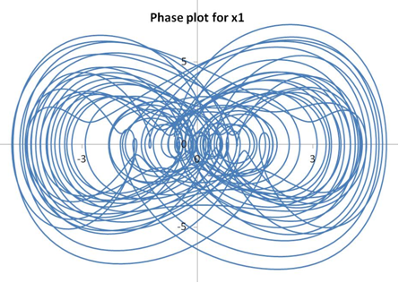
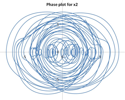
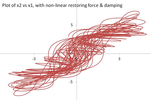
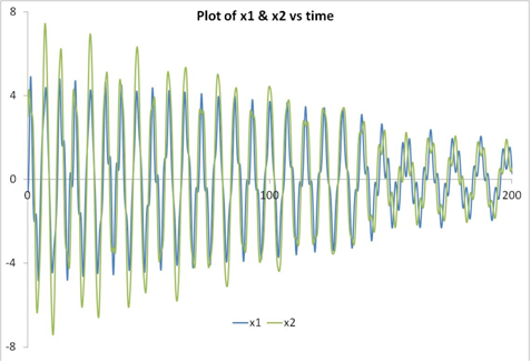
The patterns for this set of ODE’s are plotted below. Damping and the non-linear spring force appear to “compete” against each other! While the damper element tends to “dampen” out the vibrations with time (i.e., have the effect of reducing the amplitude of motion of the two masses with time), the non-linear spring effects take over in the sense of randomizing the movement of the masses.

The Trapezoidal Method

The Trapezoidal method of numerical integration is based on the premise that integration (which is the area under a curve) between two points on the abscissa can be approximated by a straight line between the corresponding ordinates. Mathematically, this can be represented as follows:

 

The similarity to the Backward Euler’s method is evident. The solution of the Trapezoidal method requires an iterative procedure at each time step to arrive at a solution for yn. A root-finding algorithm once again comes in handy for this iterative process.

A simplified algorithm for the Trapezoidal method can be:

1)    % Define step size (h), initial function y(0), initial time t0, final time tf, eps
2)    nosteps = (tf – t0)/h
3)    for i ← 1 to nosteps

- Calculate derivative function f[t0,y[i]]
- Iterate until y[i] – (y[i-1] + 0.5*h*{ f[x(i-1), y(i-1)] + f[x(i), y(i)]}) < eps
- t0 ← t0 + h

4)    % Display results

 Eq. 203(a) from J.C.Butcher, Numerical Solution of ODE’s, 2^nd Edition, was solved using the Trapezoidal method. The equations for the IVP are:

 

 

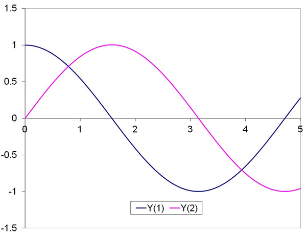
With y1(0)=1 and y2(0)= 0. A step size of 0.005, and eps of 1E-8 were used for the solver. The plots for y1 and y2 are shown below.

 

The backward Euler's method

The examples in the previous post suggested the importance of step-size ‘h’ for numerical integration, and how improper choices of ‘h’ may lead to a divergent solution. The Euler’s method presented in the former post, as indicated earlier, marched from time tn to tn+1 using the knowledge of the solution at time tn. This method is also known as the Forward Euler, since it marches forward in time.

The forward Euler at time tn uses the derivative at tn to march to tn+1. Instead, if the derivative is obtained at time tn+1, the method becomes the Backward Euler. Mathematically, it is represented by the following equation:



Since the function y(x) appears on both sides of the equation, one can no longer simply march forward between time steps. Rather, one needs to perform an iterative root-finding algorithm to determine y(x) at each time step

A simplified algorithm for the Backward-Euler can be summarized as follows:

1)    % Define step size (h), initial function y(0), initial time t0, final time tf, eps
2)    nosteps = (tf – t0)/h
3)    for i ← 1 to nosteps

- Calculate derivative function f[t0,y[i]]
- Iterate until y[i] – (y[i-1] + h*f[x(i), y(i)]) < eps
- t0 ← t0 + h

4)    % Display results

‘eps’ is a user-specified tolerance value for the root-solver. The solver iterates until the equation at each time step is less than ‘eps’. The value that satisfies this condition is the numerical solution at that time. The iteration can be performed using any root-finding algorithm like the Bisection or the Newton-Raphson method. A modified form of the subroutine ‘rtbis’ adapted from Numerical Recipes, (The art of scientific computing, Press et al, 2^nd ed.) was used for this exercise.

The Backward Euler’s method was applied to the following problem (Atkinson et al, Numerical Solution of Ordinary Differential Equations, Eg. 5.8).

 

 The solution is shown in fig. 1.

 

Euler’s method part 2- Does it work for all cases?

Let us now consider applying the Euler’s method to the problem described in Curtiss & Hirschfelder (Integration of stiff equations, Proc. of the Natl. Acad. Of Sciences, 1952, Vol. 38, pp 235-243). This is the first order DE described by the equation

 


The results of the numerical integration are shown in fig. (1) for various step sizes ‘h’, for the initial value y(0)= 1.

 

 Fig. (1): Solution of a quadratic equation for various 'h' values

Clearly the numerical solution changes for various step sizes. So which of the solution curves in fig. (1) is the “correct” solution? The simplistic marching scheme presented by the Euler’s method is clearly not “stable” for all values of step sizes. In other words, the Euler’s method does not converge to a solution for any value of ‘h’. A minimum value of ‘h’ is thus required for the numerical solutions to converge. Note on fig. (1) that the solutions tend to converge as ‘h’ decreases.


The quest for a numerical integration procedure for an ODE is thus to come up with one that is stable for any and every value of ‘h’. The forward-Euler method clearly does not appear to meet this criteria for certain types of DE’s.


To illustrate the point, the solution of the equation

 

 from Ernst Hairer & Christian Lubich, (paper titled Numerical Solution of Ordinary Differential Equations, reference unknown) for various values of ‘h’ is shown in fig. (2).

 

Fig (2): Solution for y'(x) = -50(y-cosx)

These two examples clearly illustrate the need for numerical integration techniques that can converge to a solution independent of the step size ‘h’.