The Trapezoidal Method

The Trapezoidal method of numerical integration is based on the premise that integration (which is the area under a curve) between two points on the abscissa can be approximated by a straight line between the corresponding ordinates. Mathematically, this can be represented as follows:

 

The similarity to the Backward Euler’s method is evident. The solution of the Trapezoidal method requires an iterative procedure at each time step to arrive at a solution for yn. A root-finding algorithm once again comes in handy for this iterative process.

A simplified algorithm for the Trapezoidal method can be:

1)    % Define step size (h), initial function y(0), initial time t0, final time tf, eps
2)    nosteps = (tf – t0)/h
3)    for i ← 1 to nosteps

- Calculate derivative function f[t0,y[i]]
- Iterate until y[i] – (y[i-1] + 0.5*h*{ f[x(i-1), y(i-1)] + f[x(i), y(i)]}) < eps
- t0 ← t0 + h

4)    % Display results

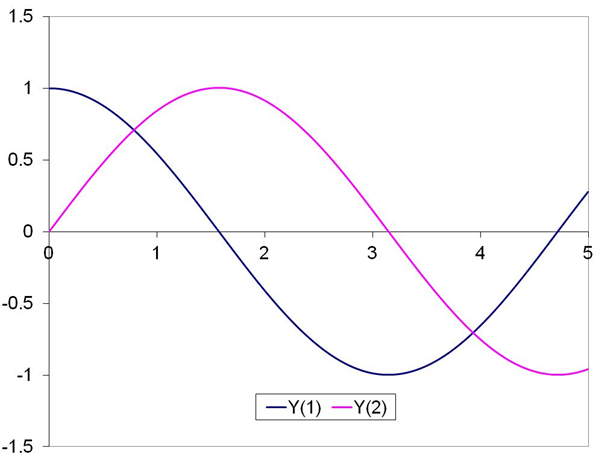
 Eq. 203(a) from J.C.Butcher, Numerical Solution of ODE’s, 2^nd Edition, was solved using the Trapezoidal method. The equations for the IVP are:

 

 

With y1(0)=1 and y2(0)= 0. A step size of 0.005, and eps of 1E-8 were used for the solver. The plots for y1 and y2 are shown below.