Coupled spring-mass system with non-linear spring

The spring forces described thus far assumed the forces to be proportional to displacement. If the spring has non-linearities in it, then the restoring force is no longer just proportional to displacement but is a squared or a cubic function. As noted by Fay & Graham, the restoring spring force can be modeled as:

The ODE's then become:

The following values were used for the simulation:

The initial values used were:

 

The patterns for this set of ODE’s are plotted below. What started as a relatively “simple” 2-DOF system has resulted in a fairly intricate displacement-web with a slight non-linearization of the restoring forces.

Coupled spring-mass-damper systems

By adding some damping to the spring-mass system, a new set of patterns start to emerge for the phase plots and the relative displacements.

The following values were used for the simulation:

The initial values used were:

 

The numerical integration was performed using the Rosenbrock triple.

A plot of displacement versus time is also shown below to better understand the physics of the motion. As expected, the oscillations tend to die down with time in the presence of viscous damping. Although the motion appears periodic and linear, it is not! And this is evident from the relative displacement plot. By merely adding damping to the system, a new pattern has emerged.

Coupled spring-mass systems

Is it possible that one does not need to resort to something as complex as a pendulum motion to create such “pretty flowers”? Can one create more such mathematical patterns by looking at simpler systems?

The motion of the pendulum is certainly complex in the real world. However, if one were to observe a ball bobbing up and down on the inner surface sphere as it traverses its motion, one may not be as “fascinated” with the actual motion, I believe. (Replace the ball with a motorcyclist and the sphere with a cage, and the motion of the motorcyclist strikes awe in every viewer, mainly due to the involvement of a human element). This is partly due to the fact that one cannot completely keep track of the entire path traversed by the mass over a substantial period of time, but rather be able to see the mass only at each instant of time. The floral pattern is nothing but a visual representation of the path traveled by the pendulum from start to finish.

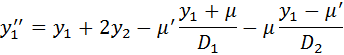
Two-degree of freedom systems with two masses connected by springs (and dampers) are a very common example taught in undergraduate mechanics courses. The equations of motion for such systems can be quite easily derived from first principles using Newton’s laws. A generalized form of the ODE’s for such a 2-DOF mass-spring-damper system is given below:





The above ODE’s are mathematically coupled, with each equation involving both variables x1 and x2. One can quite easily solve these systems of equations both analytically and numerically to obtain the position of the two masses as a function of time.

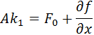
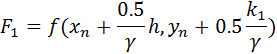
Fay & Graham (Coupled Spring Equations, International Journal of Mathematical Education in Science and Technology, 2003) present a series of examples of such coupled-spring systems. The following values were used to simulate the above equations, which were numerically integrated using the Rosenbrock triple:



The initial values used were:



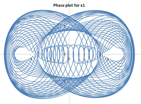
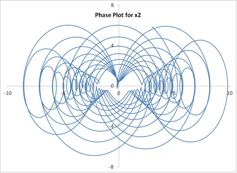
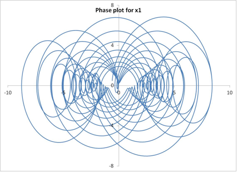
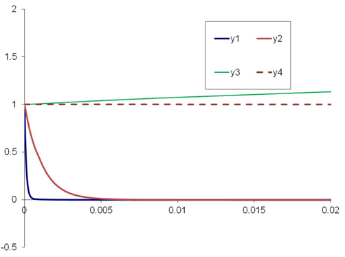
The solutions for the undamped system (ie., C1=C2=0) are shown below. The phase plot shows velocity as a function of displacement for each of the masses.




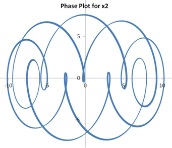
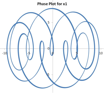
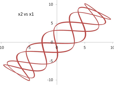
The plot of x2 vs x1 merely represents the motion of the two masses relative to each other, which would otherwise be impossible to visualize in the real world.

The Spherical Pendulum

The spherical pendulum is a generalized representation of the simple pendulum. The spherical pendulum is a 3-dimensional motion of a mass moving on the inner side of a sphere. Given an initial condition, the mass sets into motion and continues to do so in vacuum. The equations of motion for the spherical pendulum are given below.

 

 

 The Cartesian coordinates are obtained from:

 

The initial conditions of Hairer, Norsett and Wanner were used with the above equations, and were solved using the Rosenbrock Triple.

 

 The 2-D and the 3-D plots are shown below.

The 3-body orbit problem

Arenstorf orbits (ref: Hairer, Nørsett & Wanner, Solving ODEs, Vol I) refer to the special class of 3-body orbit problems that describe the astronomical motion of two bodies (with the third body restricted). The equations of motion for the restricted 3-body problem and the corresponding initial conditions are:

 

 

 

 

The Rosenbrock Triple was employed to solve the above equations. A plot of y2 vs y1 is shown below:

Numerical Jacobians

As noted in the W-method and the Rosenbrock Triple, Rosenbrock formulations require the explicit definition of the Jacobians for the ODEs. Analytical formulations for the Jacobians can be easily performed for simple ODE’s like the one presented in the examples earlier. However, the analytical definition of the Jacobians imposes a demanding restriction on the user to “create” such matrices and then program them. (Granted, one can easily avoid all the trouble of recreating the integration methodologies and resort to ODE subroutines from known sources such as Matlab, but what fun would that be…).

An alternative approach would be to numerically evaluate the Jacobians, as recommended by Shampine & Reichelt (The Matlab ODE Suite). Subroutine “fdjac” recommended by Press et al (Numerical Recipes) is one such algorithm that can be used for the numerical evaluation. “fdjac” uses a forward-difference approximation for the Jacobian calculations.

Application of the Rosenbrock Triple

The Rosenbrock triple was used to solve problem A3 from Enright & Pryce. The ODE’s are:









The initial values for all equations are 1. The Kaps-Rentrop variable step method was used, with an initial starting time of 1E-5. The solutions are plotted below.



The solutions for the equations have vastly varying settling times as noted in the plots. A zoomed-in view of the solution between times t=0 and 0.02 is shown below.



Equations y1 and y2 reach steady-state in less than 0.005 s, while y3 takes over 20 s to “settle down”. As noted earlier, such equations that have quantities with vastly varying settling times are referred to as “stiff” ODE’s. The more powerful the ODE solver, the quicker is the iterative process to converge at a solution for the entire time period of interest.

The Modified Rosenbrock Triple

Shampine & Reichelt (The Matlab ODE Suite) point out that the W-formulas can go “badly wrong when solving problems with solutions that exhibit very sharp changes”, especially within each time step. They propose a modified Rosenbrock Triple that advances between time steps. The Rosenbrock Triple is presented below, but re-written in a format that is scaled and conditioned.

       

 

 

 

 The error estimate is given by:

 

 

 

For a successful step, F2 for the completed step is the same as F0 for the next step. Shampine & Reichelt refer to it the “First Same As Last” formula, or FSAL.

The implementation of the Rosenbrock Triple is fairly straight-forward, as is obvious from the one-step formulation above. The matrix inversion in the form of LU decomposition is performed once, and the ki’s are calculated by LU back substitutions.