Matrix representation of Semi-Implicit Method

Higher order equations, or series of ODEs are more easily solved using the Semi-Implicit Method if represented as a matrix form. Thus,

 

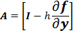
Letters in bold in the above formulation are matrix representations, and I is the identity matrix. Having represented A as a matrix, the Backward Euler can now be formulated as:

 

The matrix formulation of the Backward Euler negates an iterative process, but introduces a matrix inversion. One matrix inversion suffices for the set of ODE’s at each time step, since the partial derivatives are constant. For a set of n ODE’s, the matrix A is of size nXn, and the variable matrix yn is nX1. A matrix multiplication thus needs to be performed to determine y(n+1).

Press et al (Press, Teukolsky, Vetterling & Flannery, Numerical Recipes, The Art of Scientific Computing) recommend LU-decompositions for the matrix inversion process, followed by the LU-back substitution. Subroutines LUDCMP and LUBKSB can be implemented for this process.

The algorithm for the semi-implicit process can be summarized as:

1)    % Define step size (h), initial function y(0), initial time t0, final time tf, eps
2)    nosteps = (tf – t0)/h
3)    for i ← 1 to nosteps

-       Calculate matrix A
-       Invoke subroutine LUCDMP for A
-       B ← LUDCMP (A)
-       Invoke LUBKSB to compute h*B*f(yn)
-       f(yn) ← LUBKSB(h*B*f(yn))
-       y[i] ← y[i-1] + f(yn)
-       t0 ← t0 + h

4)    % Display results

Semi-Implicit Method Using Partial Derivatives

So, how does one avoid iterations and yet be able to solve the Backward Euler’s method? Press et al (Press, Teukolsky, Vetterling & Flannery, Numerical Recipes, The Art of Scientific Computing) suggest using a linearized form of the equation to represent the derivative f(yn+1). Using the principles of basic calculus,

 

The above representation introduces the partial derivative on the right hand side. Using this formulation and re-arranging the terms, the Backward Euler becomes:

 

For simple ODE’s that have just one equation, the above semi-implicit form can be easily solved by dividing the equation with the term in the square brackets, and then marching sequentially from one step to the next. The simplified formulation then becomes: