The Prothero-Robinson stiff ODE model

Bartel & Günther present a model for stiff systems as adapted from Kvaerno. The Prothero Robinson model that they use is defined by the following set of non-homogeneous equations:

 

The above equations represent sinusoidal solutions governed by the frequency w, with the stiffness factor governed by gamma. Bartel & Günther suggest -10E4 for the stiffness factor, with zero initial conditions at t=0, w=100 and eps =0.1. The solutions of the ODE’s are thus two variables with vastly differing settling rates, clearly justifying the classification as stiff. 

Plotted below is the solution obtained using the Generalized Rosenbrock Algorithm with the VELDS parameters.

 

Hairer & Wanner’s Brusselator problem

A good test of the Rosenbrock methods can be applied to the PDE from Hairer & Wanner. The PDE’s for the diffusion equation (also known as the Brusselator in one spatial coordinate) are:

 

The initial & boundary conditions are:

The first step in the solution of this PDE is to convert it into equivalent ODE’s, with the use of the finite difference technique & the MOL. Here is the procedure to solve the PDE’s:

• Choose the number of grid points N to be used for the finite difference method.

• Calculate the discrete location of the points on the grid:

•  Calculate the spacing between the grid points 

•  Use the finite difference technique to represent the 2^nd order PDE’s as ODE’s

 

•  Use the MOL to convert the PDE’s to ODE’s

•  Solve the ODE’s in the above step. The Rosenbrock technique with the Kaps-Rentrop GRK4A coefficients was employed in this case, with N= 40.

Plotted below are the 3D solutions of vectors u & v. 

 

Is the higher order Rosenbrock method worth the effort?

The obvious question that comes to mind is, with the additional rigor involved in the matrix inversion, and sometimes defining the analytical Jacobians for more exact solutions, is the higher order Rosenbrock method worth the effort. The explicit RK method is potentially a much easier algorithm to implement. But does it fare as well as the Rosenbrock method?

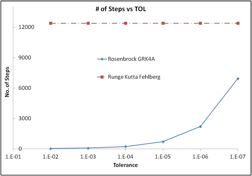
Stiff differential equations are more effectively solved with the Rosenbrock methods. Consider, for example, problem E3 from Enright & Pryce which was solved earlier. With the Rosenbrock-GRK4A coefficients, the solution is obtained from t= 0 to 500, with TOL = 1E-5 in about 715 steps. In contrast, the RK-Fehlberg algorithm takes over 12,400 steps to barely solve for the entire range.

The number of steps as a function of TOL is shown below for GRK4A for the same example. The Rosenbrock method consistently over-performs even with stringent tolerance requirements.