
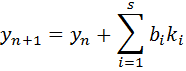
Once the ki’s are determined, the integration to the next step is achieved using
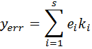
The error at each time step is given by
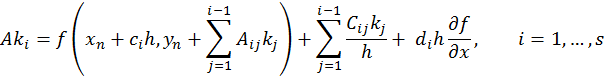
The above formulation accounts for the scaling factor by dividing the identity matrix by hγ. (ref: Shampine, Implementation of Rosenbrock methods). The Jacobian is assumed to be approximately equal to the partial derivative of the function with respect to the dependent variables (ref: Shampine & Reichelt, The Matlab ODE Suite). Much like the Generalized Runge Kutta methods, the Rosenbrock methods are also explicit single-step formulations that require an inversion of the A matrix at each time step. As indicated earlier, the LU-decomposition & LU-back substitution routines come in handy for these operations.
Similar to the RK methods, a variety of coefficients exist in the open literature for the 4th order Rosenbrock methods.
[…] ODEs, Hairer & Wanner do present the coefficients in a format that can be readily used with the Generalized Rosenbrock formulation. Adjustable step size control can be achieved using the Kaps-Rentrop algorithm. Hairer & […]
ReplyDelete[…] matrix inversion, and sometimes defining the analytical Jacobians for more exact solutions, is the higher order Rosenbrock method worth the effort. The explicit RK method is potentially a much easier algorithm to implement. […]
ReplyDelete[…] GRK4T coefficients can also be used with the generalized Rosenbrock […]
ReplyDelete