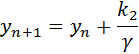
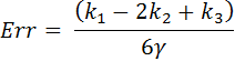
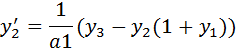
Showing posts with label Rosenbrock Methods. Show all posts

Tuesday, July 15, 2014

Kaps-Rentrop GRK4T - an example

The solution of problem B4 (class B) from Enright & Pryce was obtained using the Rosenbrock method with the Kaps-Rentrop GRK4T parameters. The ODE’s are:
  New Picture

 New Picture (1)

 New Picture (2)

 with initial conditions of y1(0)=3, y2(0)=y3(0)=0. A TOL of 1E-4 was used, with the adaptive step size algorithm. The integrated solutions are plotted below:

New Picture (3)

Monday, July 14, 2014

Rosenbrock – GRK4T parameters

Kaps & Rentrop (Generalized Runge Kutta methods of order four with stepsize control for stiff ODE’s) also provide a second set of coefficients, for gamma = 0.231. These coefficients for the GRK4T are:

A21= 0.2000000000000000E01
A31= 0.4524708207373116E01
A32= 0.4163528788597648E01
C21=-0.5071675338776316E01
C31= 0.6020152728650786E01
C32= 0.1597506846727117
C41=-0.1856343618686113E01
C42=-0.8505380858179826E01
C43=-0.2084075136023187E01
B1= 0.3957503746640777E01
B2= 0.4624892388363313E01
B3= 0.6174772638750108
B4= 0.1282612945269037E01
e1= 0.2302155402932996E01
e2= 0.3073634485392623E01
e3=-0.8732808018045032
e4=-0.1282612945269037E01
GAMMA= 0.2310000000000000
c2= 0.4620000000000000
c3= 0.8802083333333334
d1= 0.2310000000000000
d2=-0.3962966775244303E-01
d3= 0.5507789395789127
d4=-0.5535098457052764E-01

The GRK4T coefficients can also be used with the generalized Rosenbrock method.

Sunday, July 13, 2014

Is the higher order Rosenbrock method worth the effort?

The obvious question that comes to mind is, with the additional rigor involved in the matrix inversion, and sometimes defining the analytical Jacobians for more exact solutions, is the higher order Rosenbrock method worth the effort. The explicit RK method is potentially a much easier algorithm to implement. But does it fare as well as the Rosenbrock method?

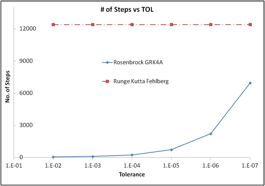
Stiff differential equations are more effectively solved with the Rosenbrock methods. Consider, for example, problem E3 from Enright & Pryce which was solved earlier. With the Rosenbrock-GRK4A coefficients, the solution is obtained from t= 0 to 500, with TOL = 1E-5 in about 715 steps. In contrast, the RK-Fehlberg algorithm takes over 12,400 steps to barely solve for the entire range.

The number of steps as a function of TOL is shown below for GRK4A for the same example. The Rosenbrock method consistently over-performs even with stringent tolerance requirements.

New Picture

Wednesday, July 9, 2014

An application of GRK4A

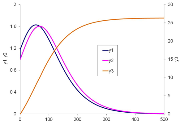
Problem E3 (stiff ODE) from Enright & Pryce was solved using the Kaps-Rentrop GRK4A parameters. The ODE’s are as follows:
New Picture

New Picture (1)

New Picture (2)

 The IV’s are y1(0)=y2(0)=1, y3(0)=0. A tolerance of 1E-5 was used.

New Picture (3)

Sunday, July 6, 2014

Rosenbrock – Kaps&Rentrop’s parameters

Kaps & Rentrop (Generalized Runge Kutta methods of order four with stepsize control for stiff ODE’s) derived a pair of coefficients based on two different values of gamma. Their original representation does not appear to account for the scaling of the identity matrix, nor does it include the coefficients for the error calculations. In their book on stiff ODEs, Hairer & Wanner do present the coefficients in a format that can be readily used with the Generalized Rosenbrock formulation. Adjustable step size control can be achieved using the Kaps-Rentrop algorithm. Hairer & Wanner’s coefficients can be found here.
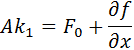
The Kaps-Rentrop coefficients for gamma = 0.395 (referred to as GRK4A) are as follows:
A21= 0.1108860759493671E01
A31= 0.2377085261983360E01
A32= 0.1850114988899692
C21=-0.4920188402397641E01
C31= 0.1055588686048583E01
C32= 0.3351817267668938E01
C41= 0.3846869007049313E01
C42= 0.3427109241268180E01
C43=-0.2162408848753263E01
B1= 0.1845683240405840E01
B2= 0.1369796894360503
B3= 0.7129097783291559
B4= 0.6329113924050632
e1= 0.4831870177201765E-01
e2=-0.6471108651049505
e3= 0.2186876660500240
e4=-0.6329113924050632
GAMMA= 0.3950000000000000
c2= 0.4380000000000000
c3= 0.8700000000000000
d1= 0.3950000000000000
d2=-0.3726723954840920
d3= 0.6629196544571492E-01
d4= 0.4340946962568634

Saturday, July 5, 2014

Autonomous vs Non-Autonomous equations

The formulation of the W-method, in its as-presented form, can be used only with equations that do not incorporate the dependent variable in them. Such equations that are functions of just the independent variables are referred to as autonomous functions.
New Picture

When the equation is a function of both the dependent & independent variables, they are referred to as non-autonomous functions.
New Picture (1)

An example of a non-autonomous ODE is the famous stiff ODE from Curtiss & Hirschfelder (Integration of stiff equations).
  New Picture (2)

Non-autonomous equations can be converted into autonomous ones by defining the independent variable as a dependent one. The above ODE then becomes:
 New Picture (3)

New Picture (4)

The above two equations can then be used with the W-method (or any method that is represented in autonomous form).

Friday, July 4, 2014

The Generalized Rosenbrock formulation

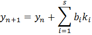
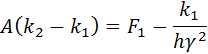
Following the methodologies outlined in Hairer & Wanner ( Solving Ordinary Differential Equations, II), the generalized formulation for the Rosenbrock methods of higher order can be stated as follows:
 New Picture
New Picture (1)

Once the ki’s are determined, the integration to the next step is achieved using
 New Picture (2)

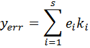
The error at each time step is given by
 New Picture (3)

The above formulation accounts for the scaling factor by dividing the identity matrix by . (ref: Shampine, Implementation of Rosenbrock methods). The Jacobian is assumed to be approximately equal to the partial derivative of the function with respect to the dependent variables (ref: Shampine & Reichelt, The Matlab ODE Suite). Much like the Generalized Runge Kutta methods, the Rosenbrock methods are also explicit single-step formulations that require an inversion of the A matrix at each time step. As indicated earlier, the LU-decomposition & LU-back substitution routines come in handy for these operations.

Similar to the RK methods, a variety of coefficients exist in the open literature for the 4th order Rosenbrock methods.

Friday, June 27, 2014

The Spherical Pendulum

The spherical pendulum is a generalized representation of the simple pendulum. The spherical pendulum is a 3-dimensional motion of a mass moving on the inner side of a sphere. Given an initial condition, the mass sets into motion and continues to do so in vacuum. The equations of motion for the spherical pendulum are given below.
 New Picture

 New Picture (1)

 The Cartesian coordinates are obtained from:
 New Picture (2)

The initial conditions of Hairer, Norsett and Wanner were used with the above equations, and were solved using the Rosenbrock Triple.
 New Picture (3)

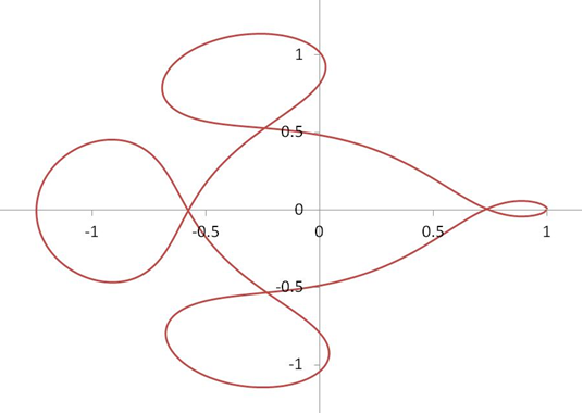
 The 2-D and the 3-D plots are shown below.

New Picture (4)


New Picture (5)

Wednesday, June 25, 2014

The 3-body orbit problem

Arenstorf orbits (ref: Hairer, Nørsett & Wanner, Solving ODEs, Vol I) refer to the special class of 3-body orbit problems that describe the astronomical motion of two bodies (with the third body restricted). The equations of motion for the restricted 3-body problem and the corresponding initial conditions are:
 New Picture
New Picture (1)

New Picture (2)

 New Picture (3)

 New Picture (4)

 New Picture (5)

The Rosenbrock Triple was employed to solve the above equations. A plot of y2 vs y1 is shown below:

New Picture (6)

Monday, June 23, 2014

Numerical Jacobians

As noted in the W-method and the Rosenbrock Triple, Rosenbrock formulations require the explicit definition of the Jacobians for the ODEs. Analytical formulations for the Jacobians can be easily performed for simple ODE’s like the one presented in the examples earlier. However, the analytical definition of the Jacobians imposes a demanding restriction on the user to “create” such matrices and then program them. (Granted, one can easily avoid all the trouble of recreating the integration methodologies and resort to ODE subroutines from known sources such as Matlab, but what fun would that be…).

An alternative approach would be to numerically evaluate the Jacobians, as recommended by Shampine & Reichelt (The Matlab ODE Suite). Subroutine “fdjac” recommended by Press et al (Numerical Recipes) is one such algorithm that can be used for the numerical evaluation. “fdjac” uses a forward-difference approximation for the Jacobian calculations.

Sunday, June 22, 2014

Application of the Rosenbrock Triple

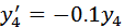
The Rosenbrock triple was used to solve problem A3 from Enright & Pryce. The ODE’s are:

New Picture

New Picture (1)

New Picture (2)

New Picture (3)

The initial values for all equations are 1. The Kaps-Rentrop variable step method was used, with an initial starting time of 1E-5. The solutions are plotted below.

New Picture (4)

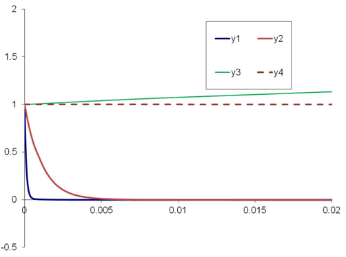
The solutions for the equations have vastly varying settling times as noted in the plots. A zoomed-in view of the solution between times t=0 and 0.02 is shown below.

New Picture (5)

Equations y1 and y2 reach steady-state in less than 0.005 s, while y3 takes over 20 s to “settle down”. As noted earlier, such equations that have quantities with vastly varying settling times are referred to as “stiff” ODE’s. The more powerful the ODE solver, the quicker is the iterative process to converge at a solution for the entire time period of interest.

Wednesday, June 18, 2014

The Modified Rosenbrock Triple

Shampine & Reichelt (The Matlab ODE Suite) point out that the W-formulas can go “badly wrong when solving problems with solutions that exhibit very sharp changes”, especially within each time step. They propose a modified Rosenbrock Triple that advances between time steps. The Rosenbrock Triple is presented below, but re-written in a format that is scaled and conditioned.
New Picture (1)

        New Picture (2)
 New Picture (3)

 New Picture (4)

 New Picture (5)

 The error estimate is given by:
 New Picture (6)

 New Picture (7)

 New Picture (8)

For a successful step, F2 for the completed step is the same as F0 for the next step. Shampine & Reichelt refer to it the “First Same As Last” formula, or FSAL.

The implementation of the Rosenbrock Triple is fairly straight-forward, as is obvious from the one-step formulation above. The matrix inversion in the form of LU decomposition is performed once, and the ki’s are calculated by LU back substitutions.

Monday, June 16, 2014

The Oregonator

The Oregonator is a series of ODE’s describing a chemical reaction for ions. The general form of the ODE’s are (ref: Haiere, Norsett & Wanner, Solving ODE’s, part I):
 New Picture

 New Picture (1)

 New Picture (5)

 The Oregonator is a set of stiff ODE’s that have significantly different settling times for each of the variables, thus making it numerically challenging to solve. The W-method with the error estimate and the adaptive step-size control was put to test to solve the Oregonator problem with the following values:
 New Picture (3)

The initial values used were y1(0)=y3(0)=400, y2(0)=1. The solution is shown below with a log-scale for the ordinate.

New Picture (4)