The Butcher Tableau for the SDIRK Method

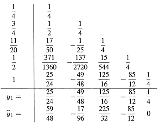
An L-stable Butcher tableau for the SDIRK method of order-4 as derived by Hairer & Wanner is shown below.

 

The implementation of the SDIRK coefficients now becomes straight-forward, with the Generalized RK formulation.

As a side note, is the lower-diagonalized method a semi-implicit method? Or is it semi-explicit? Dr. Butcher’s slides have a rather humorous take on this subject.

 

Implicit RK Methods:

My previous post touched on the differences between Implicit & Explicit methods. Implicit methods (such as the backward Euler’s method) require an iterative procedure at each step to arrive at a solution before proceeding to the next time step. The advantage, however, is that implicit methods are truly stable methods. Irrespective of the time step, convergence with Implicit methods are much better compared to Explicit ones.

A higher order Implicit-RK (IRK) method can be represented in the following form (Atkinson et al):

The result of the summation of all cj terms for each ki is a square-matrix of ALL terms (as opposed to just the lower triangular matrix with the case of an Explicit RK method). The Butcher tableau for the Implicit method thus takes the form:

 

For example, the ki terms for a 2-stage IRK method would be:

 

A Newton-type iterative solver would have to be employed to solve the above set of equations to obtain k1 & k2. In general, an s-order system will require the solution of ns coupled equations (Hairer & Wanner). On equations of several orders of magnitude, this can significantly slow down the process. Unless the set of equations to be solved are considerably stiff, where it becomes a choice between stability vs execution time.

 

Generalized Runge Kutta Formulation

For RK methods of order 4 and higher, the inter-stage vectors (k’s) can be represented using the following formulation (Atkinson et al, Numerical Solution of ODE’s):

    

The solution at t(n+1) is given by

 

J.C. Butcher (Numerical Methods for ODE’s, 2^nd Edition) invented the “Butcher tableau” methodology of representing the coefficients a(i,j), b(j) and c(j) for the Runge Kutta methods. The general format of such a tableau is

 

 The Butcher tableau for the most popular RK4 method thus becomes:

                                                                                                           

The use of the Butcher tableau, along with the generalized formulation from Atkinson, provides an easy methodology for numerical integration of ODEs.